In its most simple form, Direction aims to answer the question: within a single bar, will the Close be higher or lower than the Open? Magnitude attempts to answer the question of what will the High and Low be? It should at a minimum be able to answer what the difference between High and Low is, but the more specific, the better. One attempt at this is to explore the ratio between High-Open and Open-Low, or MFE/MAE. Understanding these bounds helps to clarify where a stop loss should be, which ultimately determines Risk:Reward.
Part I: Minimum Average Daily Range (ADR)
For this project, the target “goal” for what a successful ADR indicator looks like is based on its accuracy to predict minimum ADR. To start, I looked at the rolling average of the range for the past 10-80 days. The accuracy for this is actually quite low (37-42%), suggesting that mean>median, and thus the true distribution of ADR is tailed towards higher numbers (which is not very surprising). To get better accuracy, I halved the rolling range, and with an average range of the past 20 days / 2, the accuracy is about 94%.
ADR 20 (not divided by 2)
mean        0.008966
std         0.002554
min         0.004384
25%         0.007157
50%         0.008394
75%         0.010526
max         0.016954
Part II: Maximum Average Daily Range
Although black swan and other news impact days can cause the maximum range to be very large, it is worth looking at none the less.
75th percentile: 0.01062
80th percentile: 0.01161
85th percentile: 0.01243
90th percentile: 0.01423
95th percentile: 0.0175
100th percentile: 0.05167
At the 95th percentile, the range is only 175 pips or 33% of the max. This means that as we get closer to the max, the distribution is still following a somewhat normal curve, and really goes crazy in the last 5%. Another way of looking at it is that 175 pips is a little more than 2x the median, but the max is over 6x.
Part III: Using current ADR as an indicator of future ADR
If we follow the theory that the markets expand and contract, we should be able to find a relationship between low current ADR and higher future ADR, and vice versa. To explore this, I created a new indicator.
MFE Ratio: By assuming perfect knowledge and taking the direction out of the equation for a minute, I define MFE as whatever direction is largest. Using a combination of the past/future MFE movement, current days range, and a rolling window (by hour), I constructed a normalized indicator that measures MFE over time.
Now to explore the usefulness of the indicator, I measured the probability that the future MFE ratio is larger than the past MFE ratio. While it is clear that 50% means there is no edge, it’s also important to take opportunity frequency into account. That is if we can predict future MFE based on past MFE, does that edge occur often enough to take advantage of it?
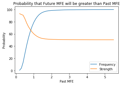
The orange line is showing that as the Past MFE/ADR ratio gets bigger, the probability that the Future MFE ratio will be bigger than the Past MFE ratio decreases and levels out at 50% (random). Likewise, the blue line is a cumulative probability showing how frequent the MFE/ADR ratio is as it grows. My key idea here is to find the intersection of decent probability and high strength. Of interest are:
Boundary line 0.3- Total Frequency: 3.74% Strength: 91.94%
Boundary line 0.4- Total Frequency: 13.29% Strength: 90.79%
Boundary line 0.5- Total Frequency: 27.53% Strength: 85.05%
The accuracy(strength) is not that much different between 0.3 and 0.4, but the frequency is much better. This boundary line is interpreted as follows:
about 13.29% of the time, the past MFE/ADR ratio is 40% or less. When this occurs, the probability that the future MFE/ADR ratio is greater than this is about 90.79%.
So we can accurately know if Future MFE>Past MFE, but to what degree?

We find that the difference between 0.4 and 0.5 is 5% in predicting if Future>Past, but it is closer to 10% when it comes to determining the degree. Example: If Past MFE is 0.4 or lower, we can expect that Future MFE to be 1.5x that past MFE about 73% of the time. However, when we raise that bar to 0.5, the probability decreases to 60%.
| Multiplier | 0.4 Bound | 0.5 Bound |
| 0.05 | 84.83 | 85.11 |
| 0.1 | 68.56 | 69.37 |
| 0.15 | 53.64 | 54.45 |
| 0.2 | 41.03 | 41.97 |
| 0.25 | 29.39 | 30.49 |
| 0.3 | 20.48 | 21.51 |
| 0.35 | 12.82 | 14.21 |
| 0.4 | 8.72 | 9.49 |
| 0.45 | 5.69 | 6.27 |
| 0.5 | 3.2 | 3.7 |
Finally, I looked at the projected Future MAE. This is effectively a measure of maximum SL, which is very useful. This also makes sense in the context that when Future MFE is increasing, and the market is likely to move from consolidation to expansion, the movement is more directional (less choppy) and as a result, the movement in the non-dominant direction is also lower. Once Past MFE is less than the 0.4 boundary, there is only a 3.2% chance that Future MAE is greater than 50% of the current MAE. This is all fairly complicated to visualize but conceptually very useful.
To summarize – we can find evidence that market ranges expand and contract, and that low ranges lead to an increased probability in high ranges. Directional markets have lower MAE and higher MFE, and by proxy higher MFE/MAE ratios. Therefore in blind risk-reward calculation scenarios excluding direction, that ratio is lowest during these periods.
