I consider wave analysis is the primary driver for direction. Because it is built on top of the current time frame, it is always contextualized and takes in as many bars as it needs to. Of course, while the “correct” wave formula is heavily up for debate and having a bad wave formula can make or break the model, each wave must work for the individual trader. Here I present just 1 wave model that I find intuitive.
Core Components:
When working with wave models, I consider it a balance between bugs and feature. By nature, a wave indicator is a lagging indicator. While it repaints by necessity, the frequency and timing of which it does determines how buggy the indicator is. Features of the indicator contain information about what direction price is likely to go next.
Model Theory:
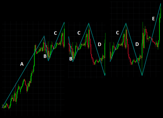
The basis of the wave model I’m going over today is built on Rolling Average Daily Range (RADR). I took the average range (daily) over 25 days and cut that number in half. Whenever price makes a move in a direction that is at least that large, it paints a new ‘leg’. A series of legs makes a wave. The logistics of the waves vary by how a trader assesses moves by High/Low vs Close, but I’ve always used Highs and Lows and always used this way of labeling swings:
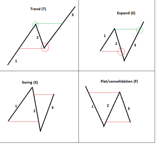
Trend: The classic ABC or 123 series. In a bullish context, the low of the 2nd leg goes no lower than the low of the 1st leg, and the following 3rd leg ends higher than the high of the 2nd leg
Expand: Each leg ends longer than the leg before it. Here the 2nd leg is lower than the low of the 1st leg, and the high of the 3rd leg is higher than the high of the 2nd leg
Swing: The middle leg is the longest leg, and 1st the first nor 3rd legs extend lower or higher respectively
Flat: The opposite of the expansion leg, each leg becomes shorter and shorter, with the high of the 2nd leg lower than the high of the 1st, and the low of the 3rd leg higher than the low of the 2nd
Mapped Model Results
Wave Leg Type Frequency:
For this particular wave model, the total frequencies end up looking like this (built on H1 time frame EUR/USD for the past ~3 years of data):
T count: 33.44%
E count: 15.77%
S count: 33.57%
F count: 17.23%
As it might be obvious, knowing what leg or series of legs is likely to occur next is a huge potential edge. Since the Trend leg is the easiest and most natural to trade, the frequency that it occurs determines, more or less, how easy it would be to trade based on the model. There are two basic approaches to this. The first is a simple “next possible leg” approach. Since legs have to be connected, not every leg can follow after any leg. For example, A Trend leg cannot be followed by a Flat leg.
Following Single Leg Frequency Distribution:
Following E:
S: 77.42%
E: 22.58%
Following S:
T: 61.17%
F: 38.83%
Following T:
S: 63.52%
E: 36.48%
Following F:
F: 24.63%
T: 75.37%
To take things a step further, one of the things I look at first is taking the complete chain of legs, and slice them up by where the Trend legs fall. By tracking legs from Trend leg to Trend leg, it can create a better picture of how typical price movement might be made.
Thus:
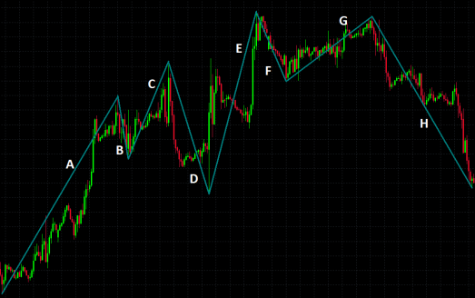
Becomes parts:
ABC = T BCD = E CDE = E DEF = S EFG = F FGH = T
The total in this set contains TEESFT.
How often does a series like TEESFT occur?
Wave Series Frequency:
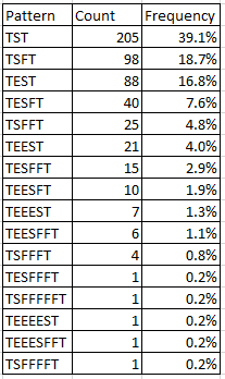
While TST is the most simple and frequent occurrence, TEST and TSFT are also common, and together are almost as common as TST. Additionally, since each additional swing leg effectively “flips” the direction that the next leg is going in, all odd number sequences are continuation patterns, and all even number sequences are reversal patterns. The net distribution is:
Continuation: 301 (56.79%)
Reversal: 229 (43.21%)
What this really means is that once the second leg is established, the probability that price will continue in its original trajectory is ~57%. The net default edge in this model is 7% better than random chance. This is one of my most robust findings, as 2-3 other models built on different origins have always resulted in a number close to this default 57%.
I’ll wrap up with a few other numbers that shouldn’t need much explanation. However, I think to really make use of this, the other areas of Magnitude and Timing really need to combine to form a more complete picture. The time of a swing leg is different than timing the market. It took me a while to realize that.
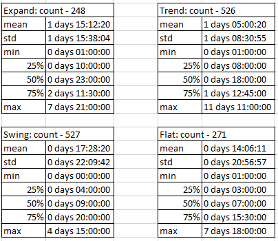
Time Duration of Each Swing:
Swing E: 1 day 15:00
Swing S: 0 days 17:30
Swing T: 1 day 05:00
Swing F: 0 days 14:00